Variable mussel production
Greenshell™ mussel production is the largest aquaculture revenue earner in New Zealand. Of this, Pelorus Sound accounts for about 68% of New Zealand’s production, where harvests are about 75,000 tonne green weight annually, generating more than $200 M per year in revenue.
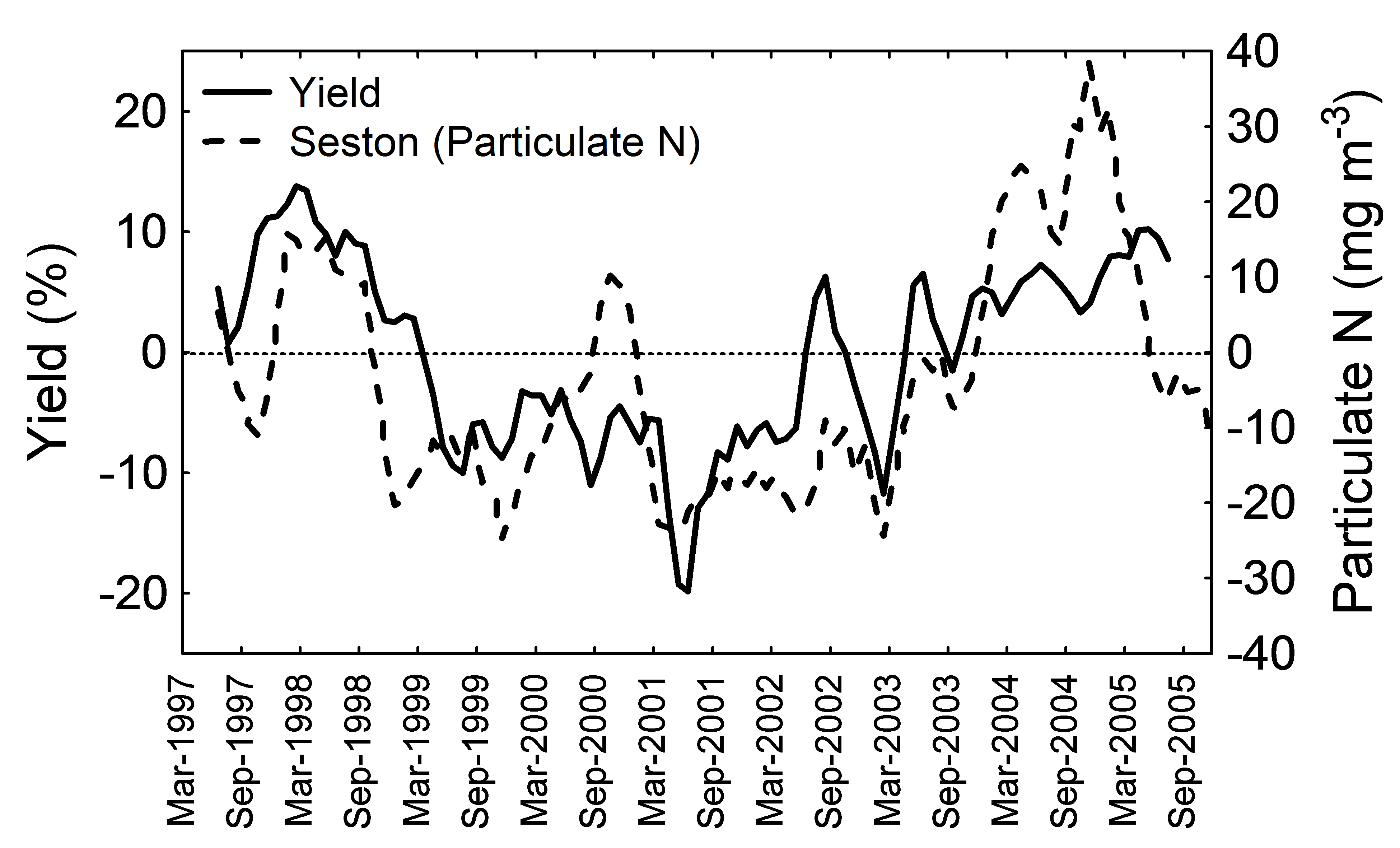
We know, however, that this production is not constant year-on-year. For example, records collected by Sealord Shellfisheries between 1997 and 2005 show a large decline and then upswing in meat yield anomaly over a six-year period, representing more than 20% variation in mussel meat production (Figure 1).
At the same time Sealord were collecting these records, the Marlborough Shellfish Quality Programme (MSQP, funded by the mussel industry and NIWA) were collecting water quality data throughout Pelorus Sound. Those data showed that the abundance of the food of mussels, seston, varied coincidentally with the mussel meat yield (Figure 1). Therefore, it was concluded that variable food supply was at the root of the variation in mussel meat production.
_Figure 1._ Variation in mussel meat yield (solid line), and their food (seston: dashed line), between 1997 and 2005, as measured by Sealord Shellfisheries and the Marlborough Shellfish Quality Programme (MSQP) programme. Data are expressed as monthly anomalies from the long-term average.
What ‘drives’ the variation?
Further investigation showed that climate is a main driver of the variation in seston availability. We found that climate conditions occurring in the summer and winter halves of the year affected mussel yields differently. The pathways by which this operates are shown in Figure 2.
Ocean upwelling is a strong driver in the summer months (October - March) because it supplies dissolved nitrogen from the deep waters of Greater Cook Strait. As these enriched waters are drawn into Pelorus Sound by estuarine circulation, it stimulates seston production, increasing mussel yield. The upwelling is driven by westerly winds in the Greater Cook Strait region, most common in El Niño summers. In contrast, La Niña summers are dominated by easterly winds, resulting in less upwelling and lower seston concentrations. Therefore, the presence of El Niño and westerly winds are strong drivers of increased mussel yield in the summer months. NIWA leverages the latest dynamical and statistical guidance to enable us to forecast the future state of the El Niño/La Niña condition with moderate confidence three months into the future.
The story in the winter months (April - September) is somewhat different. At this time of year, seston concentration and mussel yield are most strongly associated with increases in Pelorus River flow. Wetter-than-average years have more nutrients added to the sound, increasing mussel yield. The fresh water also decreases the tendency of the water column to mix vertically, enabling phytoplankton to grow better in the well-illuminated, upper parts of the water column.
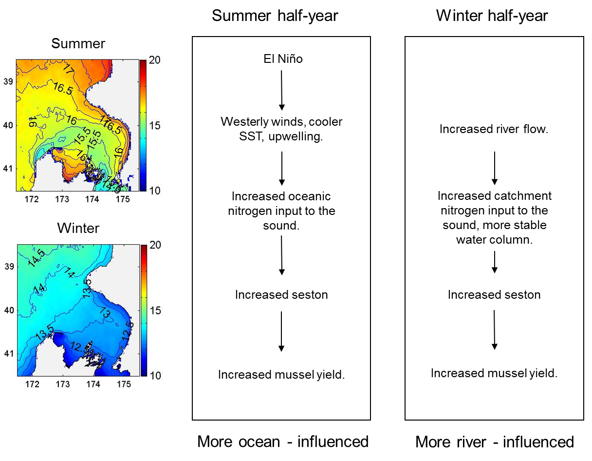
Figure 2. How climate affects mussel yield in Pelorus Sound. The left panel shows maps of sea surface temperatures (SST) derived from satellite data, in summer and winter across central New Zealand. Warm temperatures are shown by ‘warm’ colours and also higher values of the superimposed contour lines. In summer, relatively cool, upwelled waters are clearly seen in Greater Cook Strait including the area of Pelorus Sound entrance. In winter, upwelling disappears as sea temperatures cool everywhere, and waters are mixed by winter storms. The right panel describes the chain of climatic effects that drive seston concentration and mussel yield. In the summer half-year (October - March) effects are mainly from oceanic effects (El Niño, westerlies and upwelling), whereas in winter (April - September) the local effects of increased river flow become more important. See Zeldis et al. (2008) and <a href=“chiswell_GCS_upwell.pdf”, target=”_blank”>Chiswell et al. (2016) for more details.
How do we forecast mussel yield?
To create a forecasting tool, we used statistical models to combine multiple climate variables with measures of historic mussel yield. We used a historical data set of yields measured on the harvesting vessels when mussel lines were harvested between 1997 and 2005 in Pelorus Sound. We used the mussel yield observations and the coincident climate values, to find the best combination of climate variables to predict those yields. This is detailed in Zeldis et al. (2013).
In the 2013 work, we used monthly values of the El Niño-Southern Oscillation (ENSO; a measure of the strength of El Niño/La Niña conditions), wind directions and strengths from wind monitoring stations in Cook Strait (Farewell Spit and Brothers Island), satellite-derived sea temperature at Pelorus Sound entrance and gaugings of river flows measured at Bryant’s Stream in the Pelorus River. All of these data were available from international or NIWA databases for the 1997-2005 period. We then compared our predicted values of mussel yield with those actually observed, to gain understanding of the reliability by which we could predict yield from climate variables.
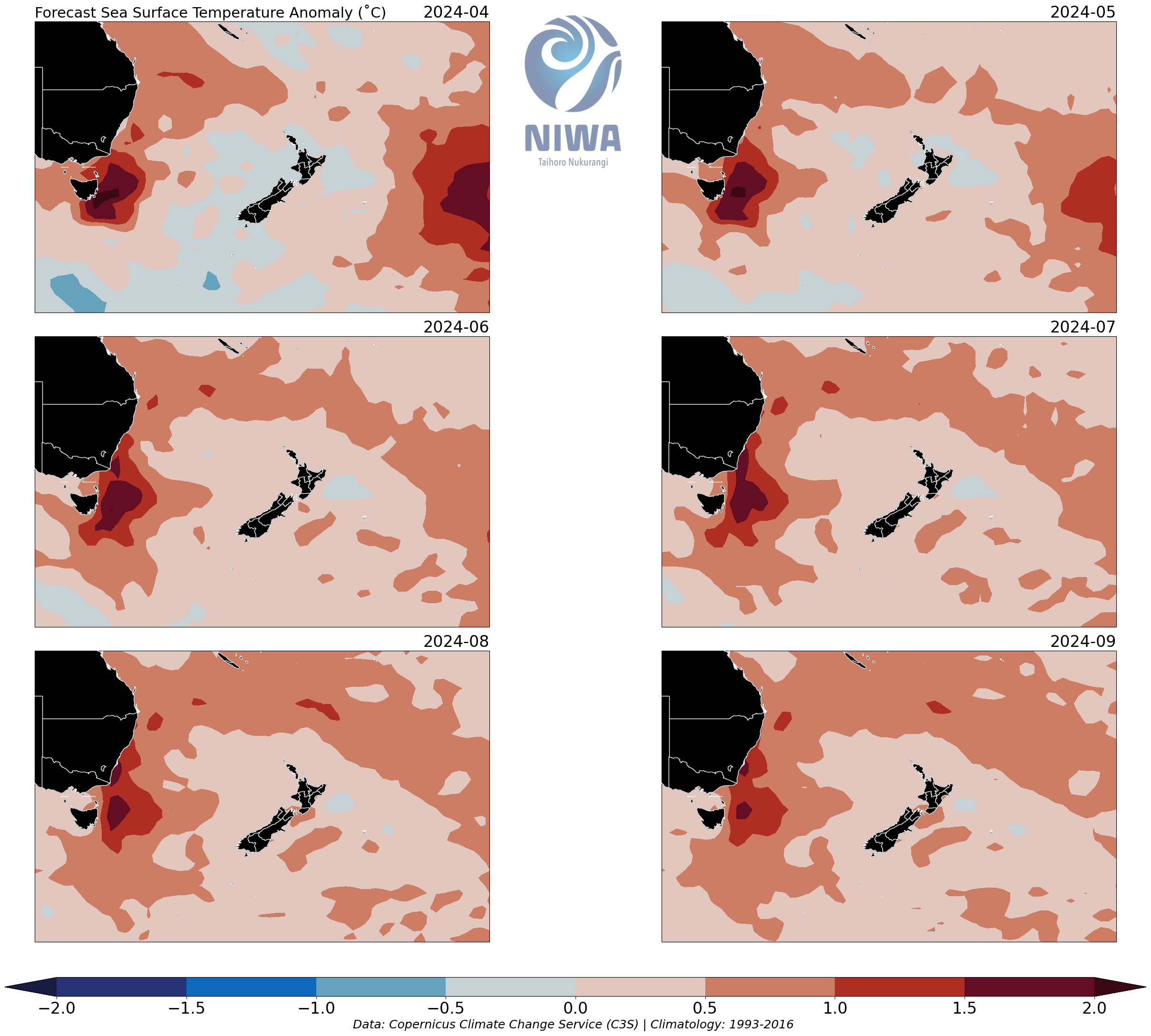
In 2022, we updated our methodology to forecast mussel yield anomalies. To identify important predictors of mussel yield we employ a data-driven approach, in which we establish relationships between mussel yield anomalies and environmental variables. These environmental variables range from wind speed to sea-surface temperature (SST). Our research suggests that SST anomalies in the Tasman Sea provide the best indicators of mussel yield anomalies. Additionally, the forecast skill from our extensive suite of international climate and oceanographical models tends to be higher for variables such as SST.
As seen in the top left panel in Figure 4, during December to February, mussel yield anomalies have a strong negative correlation with the sea-surface temperature anomalies in the Tasman Sea at latitude of approximately 45°S and a longitude of 150°E. This relationship is lagged three months, meaning that SSTs in this region 3-months prior affect mussel yield anomalies. The negative correlation indicates that warmer SSTs in the Tasman lead to negative anomalies in mussel yield in the Pelorus Sound. A change of +1°C of SST has a 15% reduction in mussel yield anomalies.
During March to May (top right panel in Figure 4), we see a similar negative correlation as December to February. Only, here we see strong correlations at lags of both 0 months instead of 3 months. A change in +1°C of SST has a 12% reduction in mussel yield anomalies.
During June to August (bottom left panel in Figure 4), mussel yield anomalies are strongly negative correlated to SST anomalies at approximately 45°S and a longitude of 155°E at a lag of 0 months. However, the sensitivity is much larger than other seasons, and so a change in +1°C of SST has a 26% reduction in mussel yield anomalies.
During September to November (bottom right panel in Figure 4), this relationship to SSTs in the southern Tasman Sea weakens. The mussel yield anomalies appear to have a stronger response to changes in SSTs near the southeast coast of Queensland (approximately 25°S, and a longitude of 155°E) at a lag of 1 month, here the correlation being positive. A change in 1°C of SST has a 12% increase in mussel yield anomalies. We also see a strong relationship between mussel yield anomalies and SST anomalies in the southern Tasman Sea (45°S, and a longitude of 155°E). This result highlights that mussels yield may respond to atmospheric teleconnections.
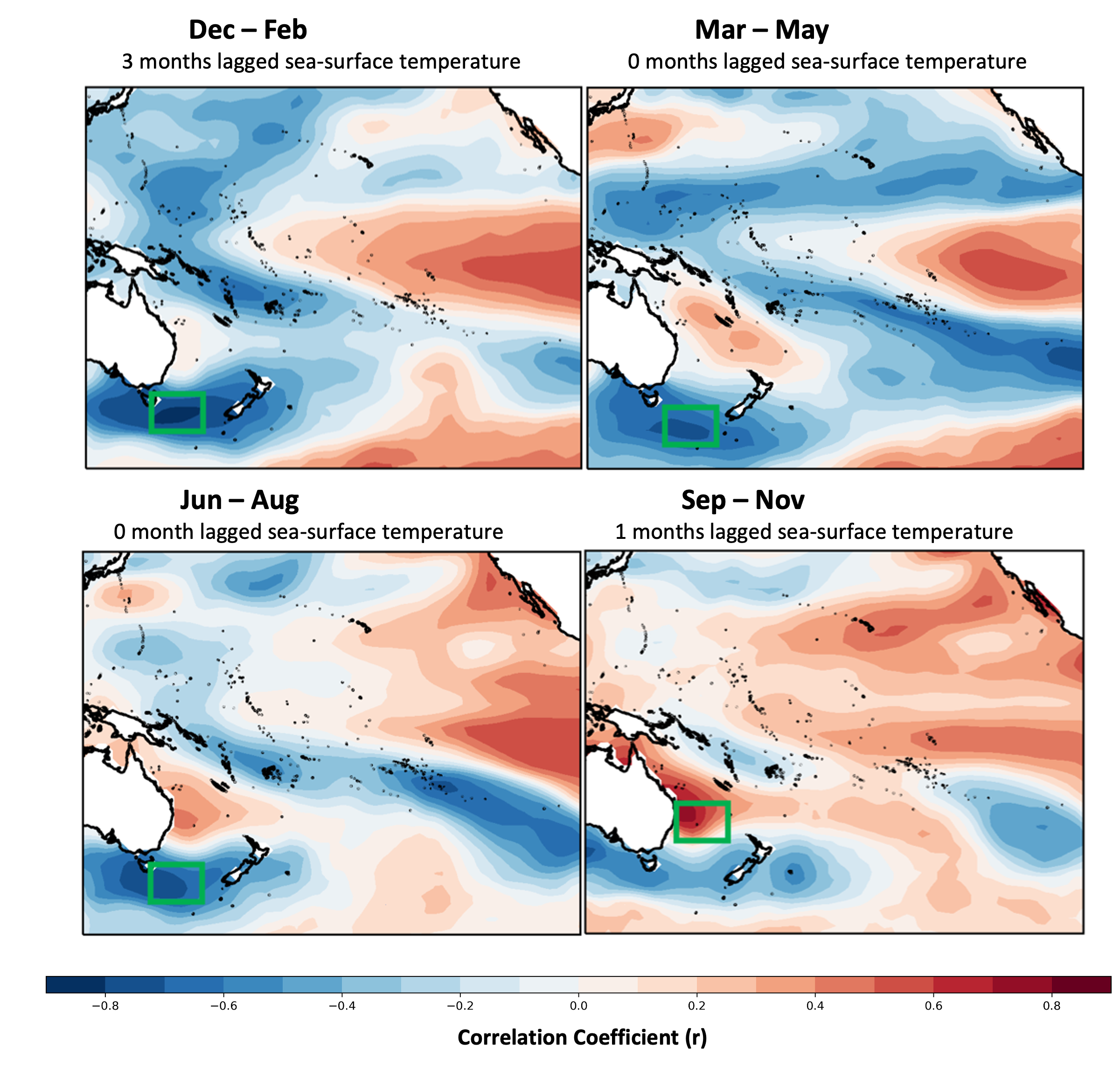
_Figure 4. Seasonal correlation coefficients for mussel yield._ Blue indicates negative correlations and red indicates positive correlations. Green squares indicate where these correlations are strongest with Pelorus Sound. The correlations have maximums at monthly lags ranging from 0 to 3 months, highlighting that significant atmospheric teleconnections may exist between these areas and Pelorus Sound. _Top left panel_ shows summer (Dec - Feb), _top right panel_ shows autumn (Mar - May), _bottom left panel_ shows winter (Jun - Aug), and _bottom right panel_ shows spring (Sep - Nov).
Validating the mussel forecasts
The validation described on this page made use of the earlier yield forecast tool. This page will soon be updated to show validation of the new forecast tool.
We can test how well our model predicts mussel yield by comparing the forecast mussel yield with yields which were subsequently observed in mussels harvested in Pelorus Sound over the relevant calendar period. Mussels were collected from Beatrix Bay every second month between August 2015 to June 2019. They were processed at NIWA, with mussel yield assessed per individual in a sample of 26 mussels with shell lengths greater than 80 mm. This work was done as part of a larger NIWA study to assess relationships between mussel body condition and environmental drivers.
We accurately predicted mussel yield 80% of the time, with the mean observed mussel yield falling within the 80% prediction interval in 12 of the 15 overlapping forecast periods (Figure 3). However, observed mussel yields were significantly lower than forecast yields between December 2015 and February 2016. The climate forecasts that we used for that period proved to be less accurate than for other periods and we believe that contributed to the larger-than-usual errors in forecasts of yield.
The mussel forecasting model uses climate forecasts to make its predictions, meaning that inaccurate climate predictions will impact our ability to accurately predict mussel yield. The 2015-16 austral summer was a period of neutral ENSO signals, making it difficult to predict the direction and strength of the climate variables used in the mussel forecasting model. For example, our climate model predicted westerly winds during this period but the observed winds were mixed. Wind direction is known to be an important driver of mussel growth in Pelorus Sound (Zeldis, Hadfield et al. 2013), with a greater proportion of westerlies leading to more seston and greater mussel growth (Zeldis, Howard-Williams et al. 2008). Therefore, it is possible that the error in predicted winds led to a lower observed mussel yield than predicted.
Despite such uncertainties, and given that we accurately predicted mussel yield 80% of the time, we have reasonable confidence in our mussel yield forecasts. The results indicate the importance of collecting mussel yield observations from the region to enable continuing validation of the predictions for model improvement.
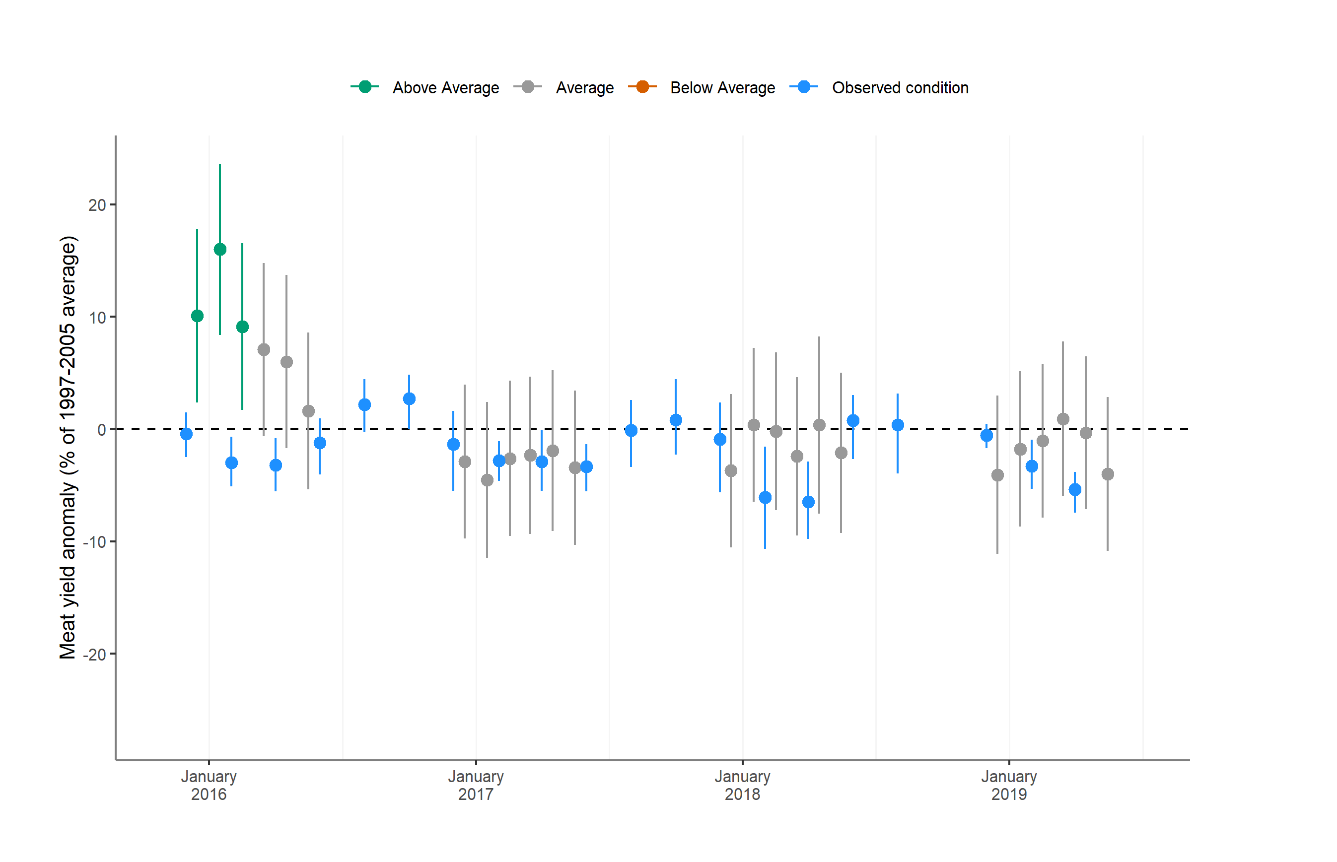
Figure 3. The relationship between forecast and observed mussel yields expressed as a percentage of the 1997 - 2005 monthly means. Forecast mussel yields (green, grey, orange) are plotted at the centre of their forecast period, with the error bars representing 80% prediction intervals. Forecast mussel yields are considered to be above or below average if the prediction intervals do not overlap zero. Observed mussel yields (blue) are plotted on the harvest date, with the solid circles and lines representing the mean yield and interdecile range (10th to 90th percentiles) for each harvest period, respectively. No forecasts were made for the winter months. Note that no forecasts of below average mussel yields (orange) were made.